
|
|
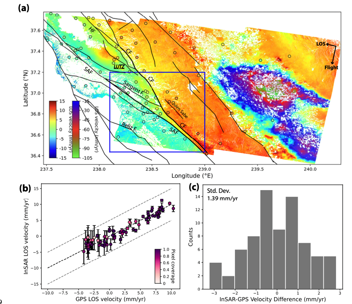
Figure 1. InSAR results and validation with GPS velocities. (a) Average 2015-2020 LOS velocity map for descending track 42. Red color indicates motion towards the satellite and blue color indicates motion away from the satellite with respect to GPS station LUTZ. Colored circles show GPS LOS velocities projected from 3D velocities estimated from the GPS timeseries during the same time period. InSAR and GPS LOS velocities are in the same color scale. Blue rectangle outlines the SAF-CF junction shown in Figure 3a. (b) Comparison of the InSAR and GPS LOS velocities. Stations within the Central Valley are excluded (Table S2). (c) Histogram of the InSAR-GPS velocity differences with a standard deviation of 1.39 mm/yr.
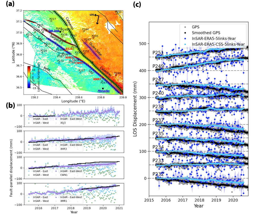
Figure 2. InSAR time series and validation. (a) Close-up view of the secular velocity field in the SAF-CF junction outlined in Figure 2a. Locations of near-fault profiles on each side of the SAF, CF, SF and QSF are shown in blue, green, brown, and purple boxes. (b) Comparison of InSAR timeseries with 3D continuous GPS timeseries relative to station LUTZ. Locations of selected stations are shown in (a). Gray dots show the raw GPS timeseries, black dots show the smoothed GPS timeseries using a 14-day moving average, blue dots show the InSAR timeseries with ERA5 weather model correction, and cyan dots show the InSAR timeseries corrected with both the ERA5 weather model and common scene stacking method (Tymofyeyeva et al., 2015). (c) Comparison of cross-fault slip inferred from InSAR timeseries (purple) with creepmeter data (black), assuming fault-parallel strike slip. The InSAR cross-fault timeseries are derived by differencing InSAR timeseries averaged in cross-fault boxes (red boxes in (a)) east (light blue) and west (light green) of the fault.
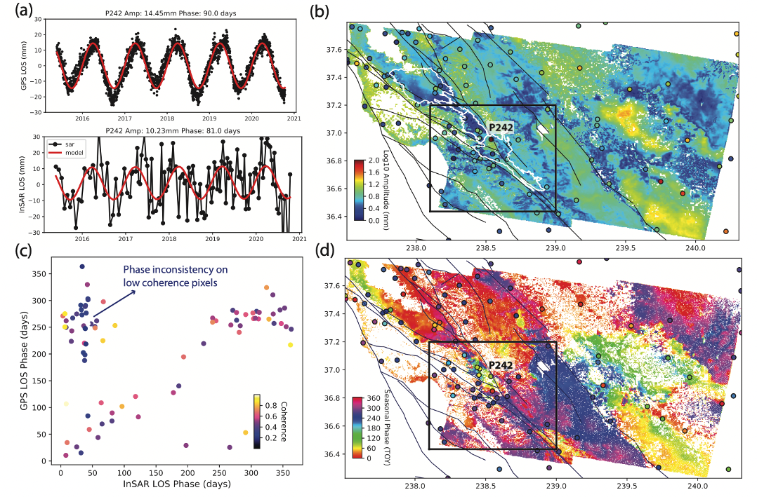
Figure 3. Evaluation of the timing of peak seasonal uplift (phase) from InSAR and LOS GPS timeseries in a North American reference frame. (a) Example of InSAR and GPS timeseries at station P242. Best-fitting seasonal sinusoidal functions are shown in red curves. (b) Amplitude and (d) timing of peak seasonal uplift (phase) map obtained from InSAR timeseries. The seasonal amplitude is shown in log scale. No phase is computed if estimated amplitude is ≤ 3 mm. Amplitude and phase values derived from GPS timeseries are shown in colored circles. Black rectangle outlines the SAF-CF junction, and white lines in (b) delineate young sedimentary basins in the vicinity of the SAF and CF faults (see Figure S7 for basin depths across the area). (c) Comparison of timing of seasonal uplift from InSAR and GPS timeseries. Each dot is colored with the average coherence from InSAR.
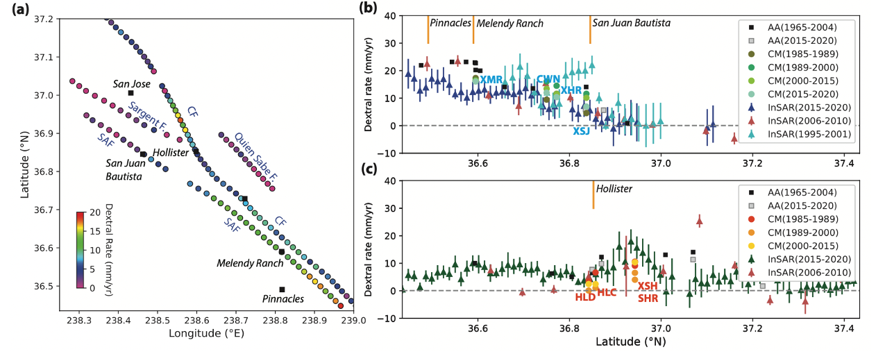
Figure 4. (a) Spatial distribution of average creep rate derived from cross-fault timeseries differences along the SAF, CF, SF and QSF (Table S3) in map view. Spatial distributions of average right-lateral creep rates along the (b) SAF and (c) CF arranged by latitude. We convert the InSAR LOS rate to right-lateral creep rate assuming all LOS motions are from horizontal fault-parallel fault creep. Blue and green triangles show the creep rates derived in this study (2015-2020) on the SAF and CF, respectively. Cyan and pink triangles show the results from InSAR during 1995-2001 (Johanson & Bürgmann, 2005) and 2006-2010 (Tong et al., 2013), respectively. Green and orange dots with different shades show the rates from creepmeter measurements during 1985-1989 (pre-Loma Prieta earthquake), 1989-2000 (post-earthquake), 2000-2015, 2015-2020, respectively. Black and gray squares show measurements from alignment arrays from multiple sources spanning 1965-2004 and 2015-2020 (McFarland et al, 2017) (Table S4).
| Project Summary | The Calaveras Fault (CF) branches from the San Andreas Fault (SAF) near San Benito, extending sub-parallel to the SAF for about 50 km with only 2-6 km separation and diverging northeastward. Both the SAF and CF are partially coupled, exhibit spatially variable aseismic creep and have hosted moderate to large earthquakes in recent decades. Understanding how slip partitions among the main fault strands of the SAF system and establishing their degree of coupling is crucial for seismic hazard evaluation. We perform a timeseries analysis using more than 5 years of Sentinel-1 data covering the Bay Area (May 2015-October 2020), specifically targeting the spatiotemporal variations of creep rates around the SAF-CF junction. We derive the surface creep rates from cross-fault InSAR timeseries differences along the SAF and CF including adjacent Sargent and Quien Sabe Faults. We show that the variable creep rates (0-20 mm/yr) at the SAF-CF junction are to first order controlled by the angle between the fault strike and the background stress orientation. We further examine the spatiotemporal variation of creep rates along the SAF and CF and find a multi-annual coupling increase during 2016-2018 the subparallel sections of both faults, with the CF coupling change lagging behind the SAF by 3 to 6 months. Similar temporal variations are also observed in both b-values inferred from declustered seismicity and aseismic slip rates inferred from characteristic repeating earthquakes. The high correlation of b-value and slip-rate changes may indicate that the SAF is extremely sensitive to small stress perturbations. |
| Tools | InSAR, GPS, Repeating earthquakes |
| Geographic Location | Bay Area, California |
| Group Members Involved | Yuexin Li <Email> <Personal Web Site> Roland Bürgmann; Taka’aki Taira |
| Project Duration | 2021 - 2022 |
| Reference | Li et al., 2022 (under review) <Preprint available!> |