
|
|
Figure 1.
Map of the greater San Francisco Bay Area with high-rate GPS stations. Lines connecting the stations indicate station pairs (172) we use in the processing. White dots are non real-time PBO stations.
| Project Summary |
In an effort to improve earthquake parameter estimation in earthquake early warning for large earthquakes (such as moment magnitude and finite fault geometry), the BSL is working to integrate information from real-time GPS and now generates and archives real-time position estimates using data from 62 GPS stations in the greater San Francisco Bay Area. This includes 26 stations that are operated by the BSL as part of the Bay Area Regional Deformation (BARD) network, 8 that are operated by the USGS, and 29 stations operated by the Plate Boundary Observatory.
Data from these sites are processed in a fully triangulated network scheme in which neighboring station pairs are processed with the software trackRT (Herring et al., 2010). Positioning time series are produced operationally for 172 station pairs (Figure 1); additional station pairs will be added as more real-time stations become available.
|
| Architecture and Data Processing |
The G-larmS architecture and process flow are depicted in Figure 2. Most notably, G-larmS consists of two independent modules for offset estimation and earthquake parameter estimation. Within these, the actual methods to get the respective values are easily exchangeable and could be easily exported to other agencies in other geographic regions.
A list of 172 station pairs (baselines) forms the basis of the Bay Area network. Each of these baselines is processed by an individual trackRT process to generate position time series. For event response and quality assessment, we consider the most recent 10 minutes of data. Multipath and other noise treatment will be implemented in the future. We categorize time series as `good' or `bad' based on a few metrics such as standard deviation over the 10 minute time window. These quality parameters are passed along with the derived offsets.
The GPS system listens to CISN ShakeAlert (Hellweg et. al., 2013) to get earthquake alarms. Once the seismic system triggers, we estimate and publish the offset evolution for a subset of baselines (see below). In parallel, the parameter estimator prepares to ingest these offsets to invert them for rupture length and magnitude.
|
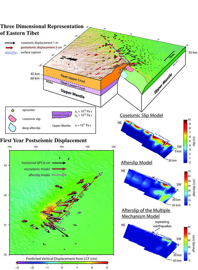
| Model of the Postseismic Displacement | The afterslip is the continuous slip of the fault after the main shock and is often considered downdip of the fault rupture zone (Wang et al., 2012). We use a dislocation model with layered structures to investigate the afterslip distribution by inverting the geodetic data. We modify the fault geometry proposed by Shen et al. (2009) and extend the fault width to 65 km depth for afterslip at the downdip extension (afterslip model in Fig. 1). The afterslip distributes on both shallow and deep parts of BCF that represents the fit to the near- and far field displacement. We use a 3D finite element model to construct a regional rheologic model composed of an elastic Tibet upper crust and Sichuan crust, a viscoelastic Tibet lower crust, and a viscoelastic upper mantle. We use the bi-viscous Burger’s rheology to represent the transient and steady state periods of the postseismic deformation. The Burger’s rheology is composed of a Maxwell fluid connected in series with a Kelvin solid to represent the steady state and transient viscosities (η1 and η2, respectively). The best-fitting model is composed of the LCF located between 45 and 60 km in depth and can produce more far field postseismic displacement. The afterslip model can explain the postseismic displacement in the near field but there is larger misfit in the far field. On the other hand, the viscoelastic relaxation model can explain the far field postseismic displacement better than the near field. It appears that a single mechanism cannot solely explain the postseismic displacement. A multiple- mechanism model is needed to fit both near- and far field displacements. We consider the 15 km thick LCF to be the main mechanism of the far field displacement, so the afterslip model may explain the misfit of the LCF model. The inversion (the 2nd afterslip model in the lower right in Fig. 1) of the LCF residual displacement shows a significant reduction of the deep afterslip. As a result, the afterslip alone model requires more than 45 cm slip in the first year below Tibet’s Moho that may already undergo ductile deformation, whereas the viscoelastic relaxation in a 15 km thick LCF can explain the GPS measurements. Consequently, the result of the Wenchuan postseismic displacement supports a weak lower crustal flow underneath eastern Tibet. |
| Tools | InSAR processing and analysis, GPS data analysis, forward and inverse elastic and viscoelastic modeling |
| Geographic Location | Eastern Tibetan Plateau |
| Group Members Involved |
Mong-Han Huang, Roland Bürgmann |
| Project Duration | In Progress: start of 2009 through 2014 |