The Cascadia Subduction zone off the west coast of Northern California, Oregon, Washington, and Britich Columbia is where the Juan de Fuce tectonic plate collides with, and sinks below, the North American tectonic plate. Subduction zones host the largest earthquakes in the world, and the Cascadia subdiction zone in particular experienced an earthquake owith an estimated magnitude of 9.0 earthquake on January 26, 1700. The expected recurrance interval for large earthquakes in this region is 300-500 years.

In beween large earthquakes, the Cascadia subduction zone is not dormant. Rather, it's home to two recently discovered phenomena: slow slip events and tectonic tremor. In a slow slip event, the deeper extent of the interface between the two tectonic plates slips, as in an earthquake, but does so more slowly. While earthquake slip occurs over the course of seconds, slow slip occurs over the course of days to weeks. The vast majority of this slip is "silent", meaning it cannot be detected with seismic instruments. But, slow slip events in Cascadia do move the surface of the earth up to 1 cm, and this movement can be detected using GPS and other instruments (Figure 1). A small percentage of the slip during slow slip events is fast enough to generate seismic waves; this is called tectonic tremor. Tectonic tremor sources can be detected and located seismically. While slow slip and tremor are not dangerous to humans or the environment, they provide a window into the physics of subduction zones. Additionally, by characterizing and monitoring slow slip events, scientists may be able to detect changes leading up to a future large earthquake.

Slow slip and tremor occur together in Cascadia at episodic intervals. Therefore, they are considered one phenomenon called Episodic Tremor and Slip, or ETS. Constraining the precise location of geodetically measured slip during ETS is important for clarifying the relationship between slip and tremor during ETS, the location of ETS slip relative to the strongly locked zone, and the role of ETS in the overall slip budget. Dr. Bartlow developed a new method for separating GNSS time series in Cascadia into ETS and inter-ETS components, deriving long-term average ETS velocities for each site. These velocities are then inverted for a time-averaged ETS slip-rate on the plate interface. ETS and its role in the slip budget is highly variable and segmented along strike. This inversion represents the highest resolution image of the ETS zone derived from geodetic data to date. Slip correlates well with tremor locations, and a possible second updip ETS zone is detected.

The regional velocity field is complex, and results from the superposition of many tectonic deformation sources, including but not limited to the Cascadia subduction zone. Most of these sources are associated with faults which are well approximated as temporally steady. The method developed here separates ETS motions from inter-ETS velocities without requiring any knowledge of the physics of the regional deformation field. It assumes only that ETS motions at GNSS stations are temporally correlated with tremor in the nearby region, and that other sources of deformation are not time-dependent during the GNSS observation period (roughly 1995 - present).

To separate ETS velocities from inter-ETS velocities, I must first identify ETS and inter-ETS periods associated with each GNSS site. I identify times of possible ETS signals at each station using a tremor catalog, available from the Pacific Northwest Seismic Network at https://pnsn.org/tremor. Each dat at each station is classified as either belonging to an ETS period or an inter-ETS period according to specific criteria. If a minimum number of tremor detections (T_min) are found in the modified PNSN tremor catalog within a specified radius (R_T) of a station for a minimum number of consecutive days (SSE_L), I classify these days as ETS periods. Data during ETS time intervals is then removed from each time series, leaving only data during inter-ETS intervals. I then fit each component of these inter-ETS only time series using least squares with equation below, which includes estimating an inter-ETS velocity (v), amplitudes of annual and semiannual seasonal signals modeled as sines and cosines (A, B, C, and D), and offsets during ETS periods (DeltaX_M).

Where N is the total number of ETS periods at this station, and H(t-t_M) represents a Heaviside step function. Once the inter-ETS velocities and seasonal terms have been determined for each component of each station, these terms are subtracted from the full length original time series. The remaining time series, should contain only deformation associated with ETS events, plus noise sources. These ETS time series are then fit with a simple line. The slope of this line across all three components at a given station defines the Long-Term Average ETS Velocity, or LTA-ETS velocity. An example of this inter-ETS velocity and LTA-ETS velocity separation procedure for station ALBH is shown in Figure 1. Figure 2 shows the resulting inter-ETS and ETS velocity fields for different GNSS processing centers, and a combined ETS velocity field.

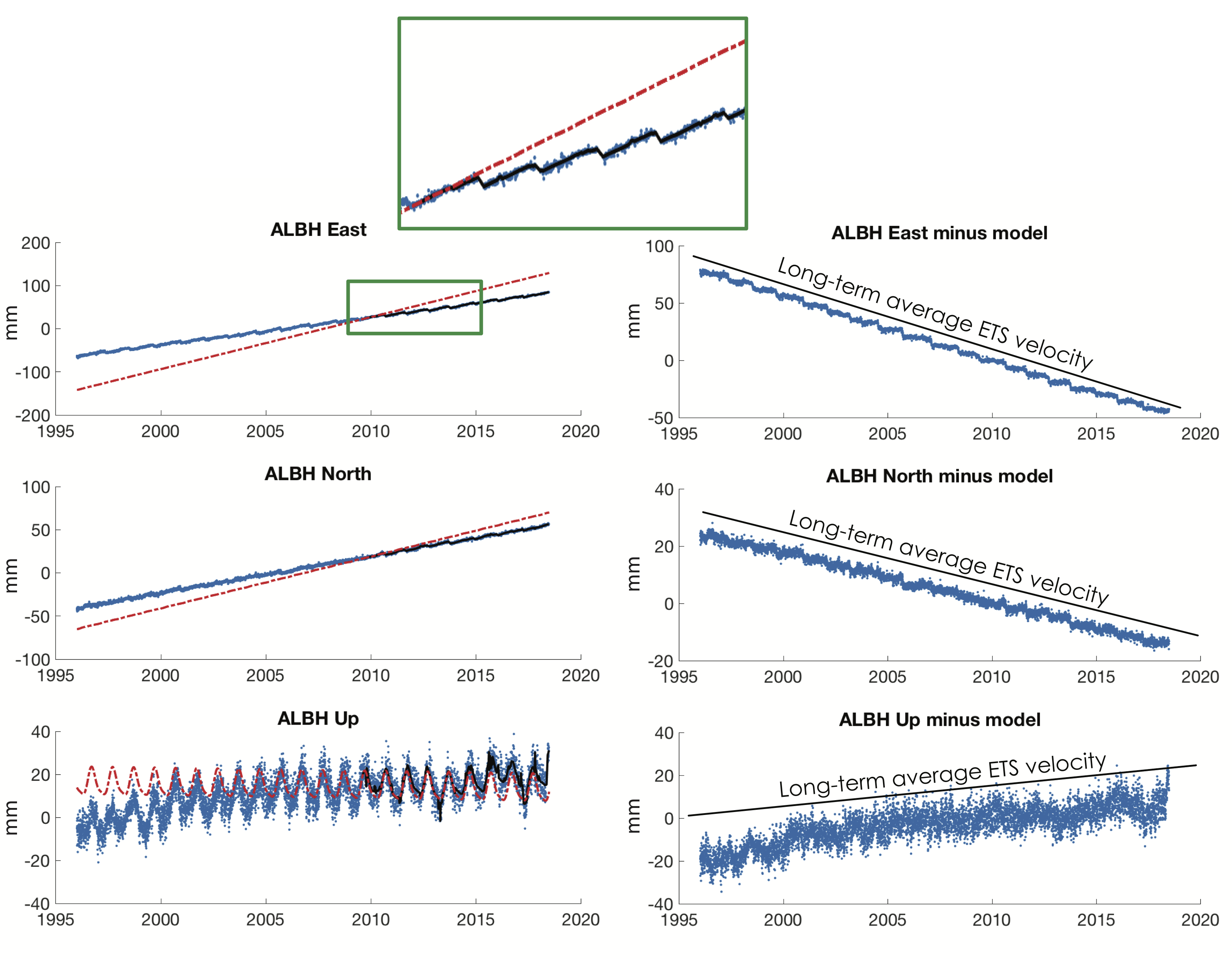Figure 1: Example of inter-ETS and LTA-ETS velocity fitting procedure for station ALBH, located on the southern end of Vancouver Island. Left: East, North, and Up time series (blue dots), shown with the fit from equation 3.1 (black line). The red dashed lines illustrate the inter- ETS velocity and seasonal terms (first six terms) from equation 3.1 propagated back in time. The E and N components include seasonal terms but they are negligibly small at this station. The red line is then subtracted from the time series to generate the figures in the right column. Enlarged green box shows a magnification of part of the ALBH East time series from the left plot, also indicated with a green box. Right: ALBH time series with the inter-ETS and seasonal terms subtracted (blue time series minus red line from left panels), leaving only ETS o↵sets and noise sources. These time series are then fit with a line, the slope of which defines the Long-Term Average ETS (LTA-ETS) velocity.

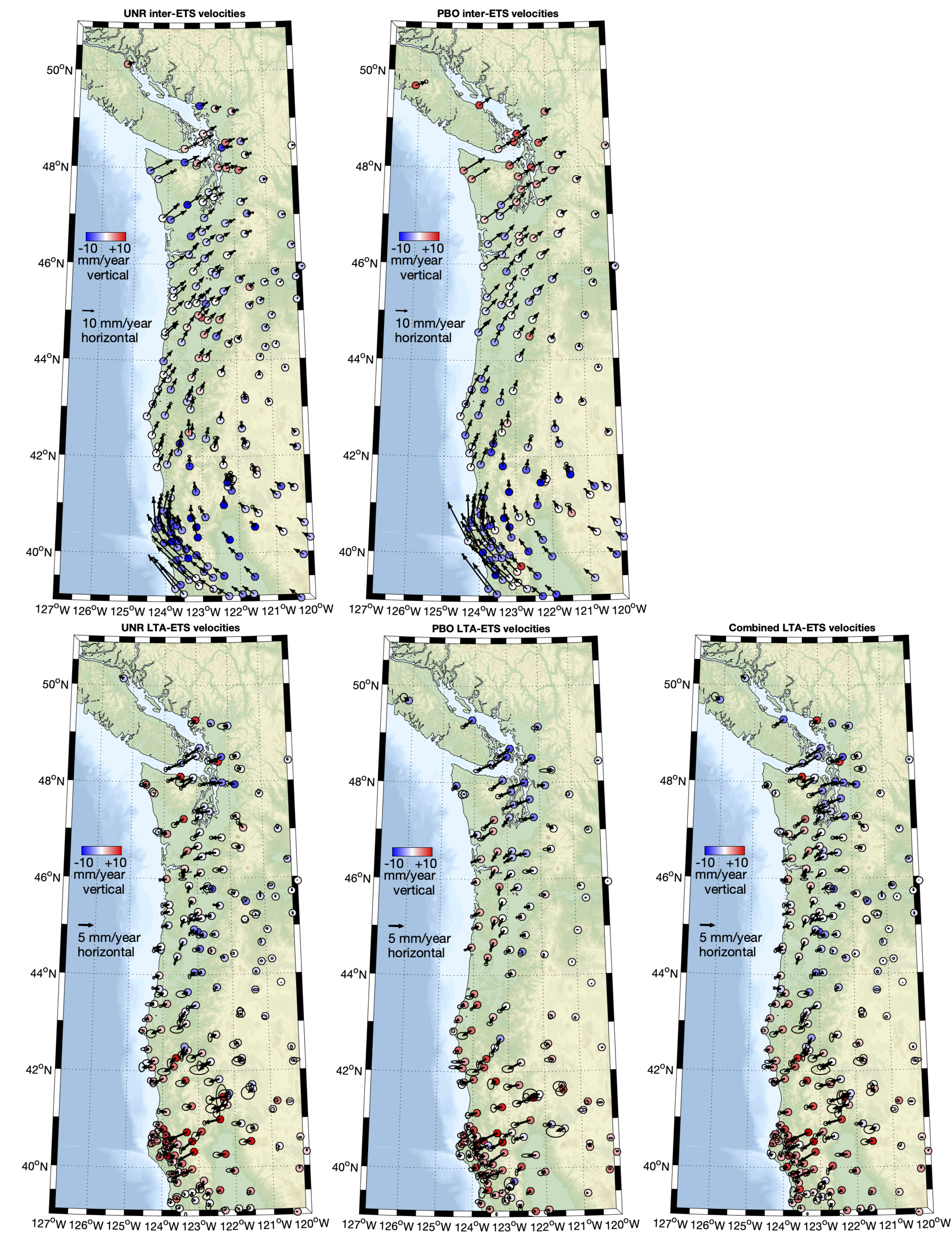Figure 2: Inter-ETS and LTA-ETS velocities for UNR and PBO datasets, and a combined LTA-ETS velocity field. All vectors have error ellipses, all though some may be too small to see.

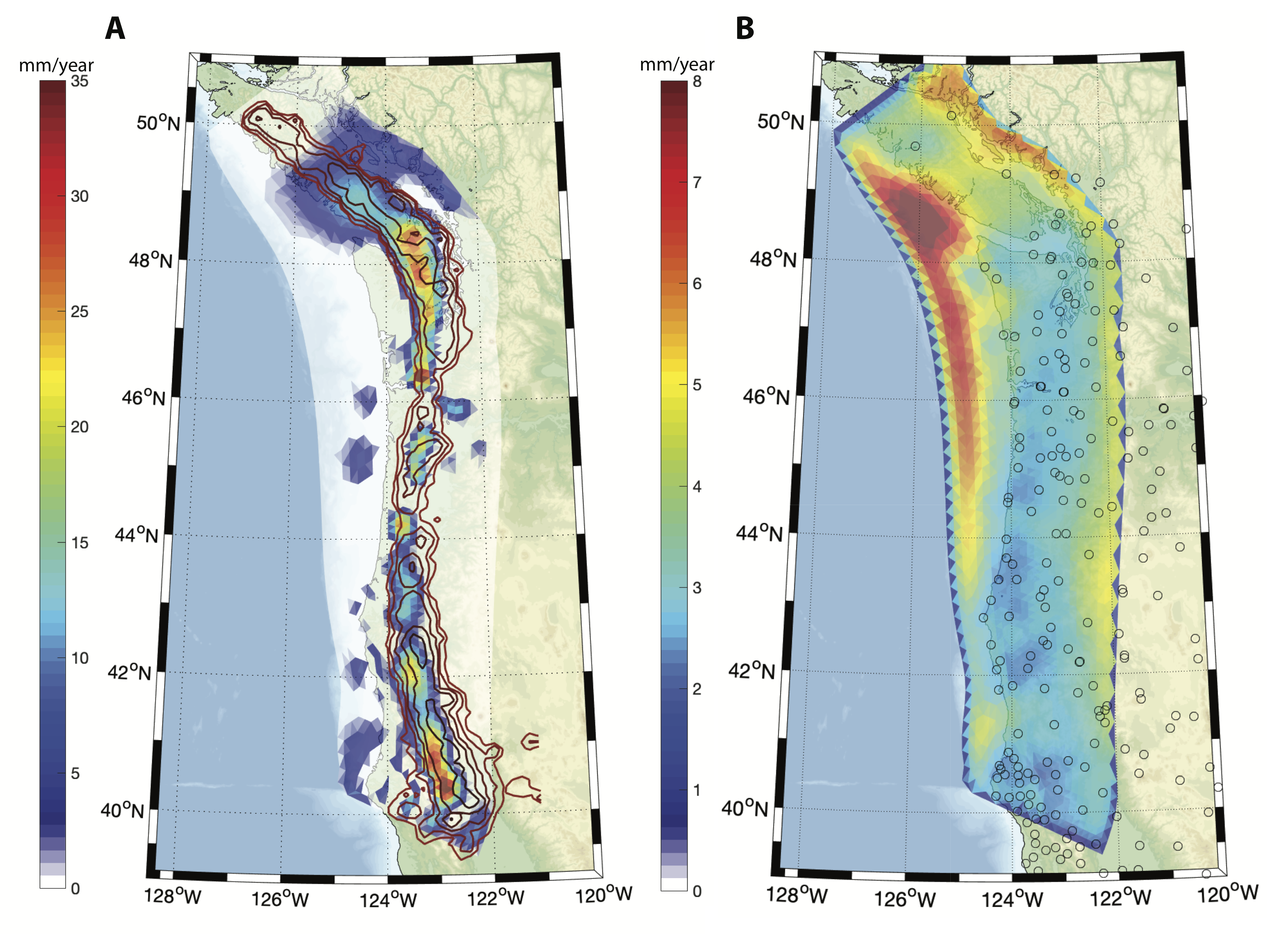Figure 3: Inversion results for the combine PBO and UNR ETS velocity field. Contours represent density of tremor detections, spaced logarithmically. A) The time-averaged ETS slip rates on the plate interface B) Slip-rate uncertainty. Note different color scale. Black circles indicate station locations.

Figure 3 shows the results of inverting the combined ETS velocity field shown in Figure 2 for slip-rate on the Cacadia subduction plate interface. Brown contours indicate density of tremor detections. This result should be interpreted as the time-average ETS slip-rate, which is directly comparable to the plate convergence rate to quantify the role of ETS slip in the overall "slip budget" of the Cascadia subduction zone. In Northern and Southern Cascadia, ETS slip accmodates 75 - 100% of the slip budget within the ETS zone, implying little to no residual locking to be released in future earthquakes or postseismic slip. In Central Cascadia, ETS slip accomodates 0 - 50% of the slip budget, depending on location. This implies either residual locking, or significant inter-ETS plate interface creep. Clearly, ETS behavior is highly variable along the subduction zone.

Figure 4 shows the fit to the LTA-ETS velocities from the preferred inversion shown in Figure 3. Circles show vertical velocities and rings around them show fit to the vertical velocities. The fits are split into the 3 segments of Cascadia for visibility. Each segment has slightly different horizontal and vertical scales. LTA-ETS velocities are smallest in the central segment and largest in the southern segment. Most horizontal model vectors fall within the LTA-ETS error ellipses, with a few outliers present in the data.

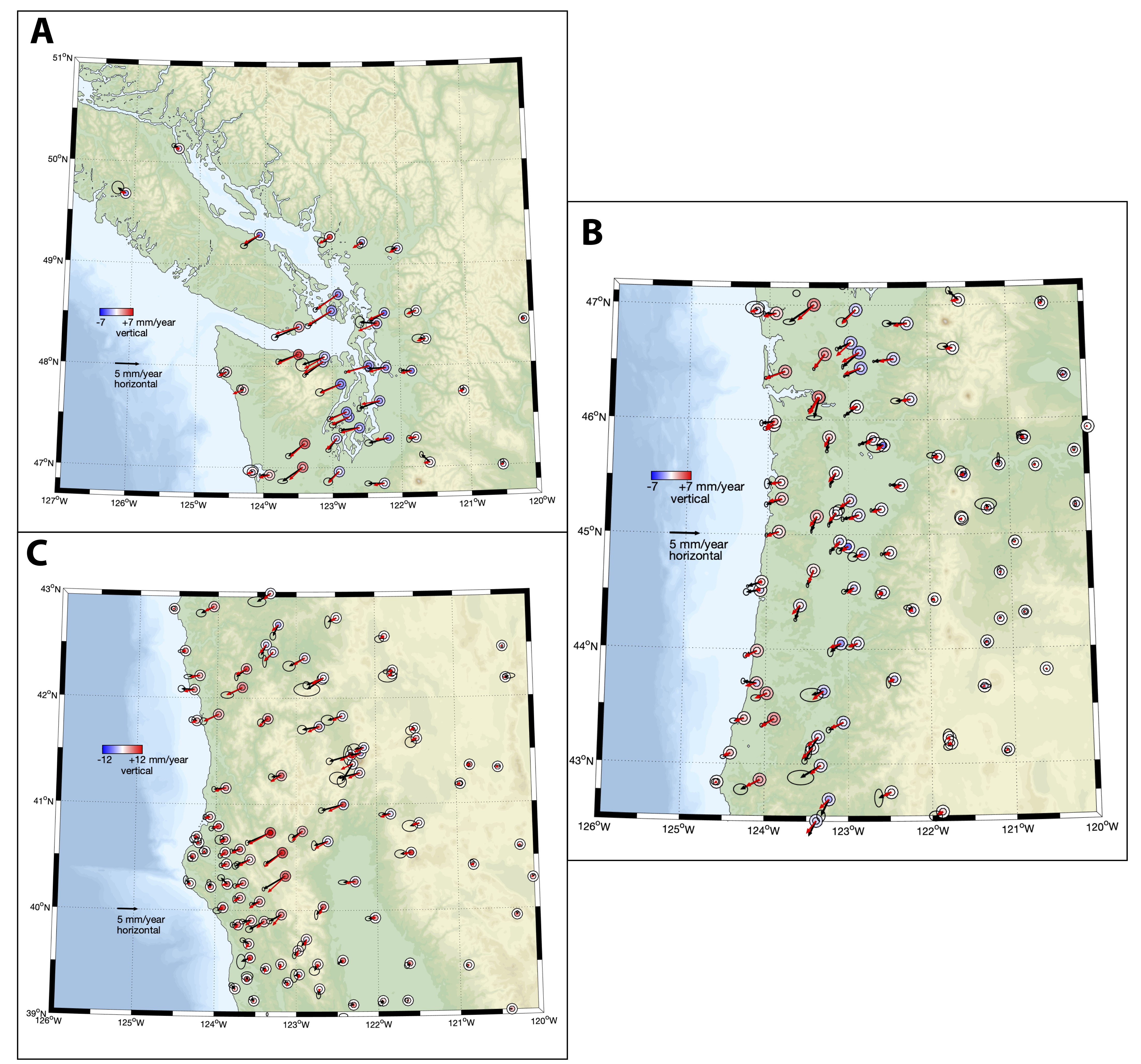Figure 4: A) LTA-ETS velocity vectors and uncertainty ellipses (black) and model fits (red) for the Northern segment. Fits shown are for the prefered model shown in Figure 3. Colored circles represent vertical velocities; rings around the circles are model fits to vertical velocities. Vertical uncertainties are not shown but are used for inversion weighting, they generally larger than horizontal uncertainties. B) Same as A, but for the Central segment. C) Same as A, but for the Southern segment.