REFERENCE MODELS

Introduction

To a very good first order approximation, the earth is made up of concentric spherical shells, and its average internal structure can be described in terms of variations of properties as a function only of depth. Measurements of travel times and amplitudes of seismic waves generated by large earthquakes and observed at distant stations contain information about the elastic and anelastic properties of the medium through which they travel. These measurements can be used to build models of seismic velocity, density, and attenuation structure with depth through mathematical inversion. Earth properties are observed to change laterally and vertically, but change most strongly with depth (lateral velocity variations are at most 10% laterally compared with 500% vertically) thus Earth structure can be well approximated by a 1-dimensional (spherically symmetric) model of elastic velocities, density, and attenuation as a function of depth (Fig. 1). Different 1D reference seismological earth models have been constructed using different data types, different parametrisation, and computation procedures. Knowing what choices have been made in the construction of a 1D seismological reference earth model is important when one wants to use such a model, depending on the application.

Figure 1 – 1-Dimensional Earth structure and velocities for the Preliminary Reference Earth Model or PREM (Dziewonski and Anderson, 1981). a. Radial Earth structure showing the major divisions. Solid lines mark discontinuities due to phase changes or compositional changes. b. Corresponding depth-dependent velocity structure for compressional and shear-waves (Vp and Vs, respectively). c. Depth-dependent density structure.

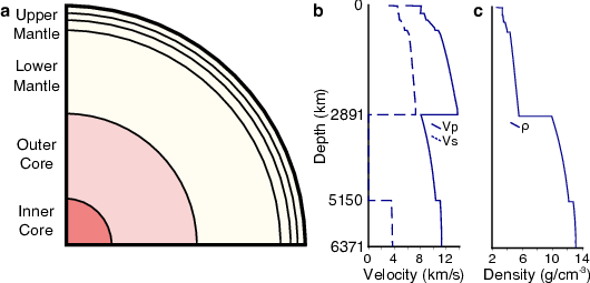
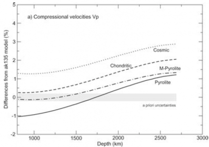
The differing sensitivities of the seismic observables used and the scatter in the measurements caused by lateral velocity structure (Fig. 2) mean that the resulting velocity structure is only an approximation of the true Earth and not representative of any real physical structure, mineral assemblage, or location. Caution must be taken when 1D reference models are used to interpret results from other disciplines, such as measurements or calculations of elastic properties of different mineral assemblages.

Figure 2. IASP91 travel-time curves with travel-times measured from test events used to verify the model. Velocity varies most strongly with depth, thus arrival times roughly follow curves with distance for each wave. However, despite the source parameters of the test events used here being well known, the scatter in arrival times demonstrates that a 1-Dimensional model is only an approximate representation of the Earth. Figure 6 from Kennett and Engdahl (1991).

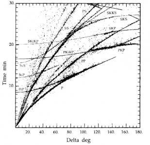
While reference models are approximations of the real Earth, they are needed for, among others, the following purposes:

• Determining earthquake locations, which involves converting times to distances and thus requires an understanding of wave propagation velocities.
• Identifying different kinds of seismic waves (phases) on seismic records is guided by calculations of predicted travel-times
• Predicting ray paths requires knowing the velocity structure
• Modelling the propagation of waves from earthquakes requires an understanding of the velocity structure
• Construction of 3D seismic models requires a starting model for the inversion process. Indeed, most of the non-linearity resides in the 1D model.
• Reference models are used to forward model standard travel-times and waveforms against which to compare observations to help identify variability
• Providing a reference for the interpretation of mineral physics experimental and computational data
• Providing a reference structure to inform dynamic modelling

Many current seismological studies rely upon reference models. While global 3D models of the Earth's mantle have been developed for over 30 years (e.g. Dziewonski et al., 1977, Dziewonski, 1984), 1D models are still commonly used.

Historical background

The earliest representation of Earth structure was a simple layered model (Table 1) derived from travel-time curves displaying how the time taken for waves to arrive following an earthquake varied with distance e.g. Gutenberg or the Jeffreys-Bullen Tables (Jeffreys 1940, Bullen 1942). These tables were compiled from observations from 1930 to 1939 when the global network of seismometers was very limited. Nonetheless, the International Seismological Centre used the Jeffreys-Bullen tables in their earthquake location process until 1991 (Kennett and Engdahl, 1991).

Region	Depth (km)	Features of region
A	33	Crustal layers
B	413	Upper mantle: steady positive P and S velocity gradients
C	984	Mantle transition region
D	2898	Lower mantle: steady positive P and S velocity gradients
E	4982	Outer core: steady positive P velocity gradient
F	5121	Core transition: negative P velocity gradient
G	6371	Inner core: small positive P velocity gradient

Table 1: Regions in Jeffreys-Bullen earth model. After Stein and Wysession (2009).

Later compilations of body wave travel-time tables determined that the Jeffreys-Bullen tables were 2-4 seconds slow and that, due to strong upper mantle heterogeneity, velocities at short distances needed revision (Herrin et al., 1968).

Constructing a model

Constructing a reference model requires a number of choices that depend on: the type of data, computational ease, and the goal of the model. Models are calculated from different datasets and frequencies and may be represented in different mathematical ways. Therefore, different models do not all represent the Earth structure in the same way.

Models are commonly constructed using either long period or short period teleseismic data (Fig. 3). Short period data are sensitive to only small volumes of the Earth thus can be biased by sampling, but can carry precise information about the Earth and are sensitive to the deep Earth. Meanwhile, long period waves are sensitive to larger volumes or, in the case of normal modes, the whole Earth. The frequencies of seismic data used to construct the model affect how the resulting model should be used. Seismic data can be supplemented by other measurements, such as astronomical data. See Table 2 and Data section for more detail.

Figure 3 – Seismic data types used to construct reference models. a. Body waves travel through the Earth, therefore, they can sample all depths although lateral resolution is limited by the location of sources and receivers. Body waves are relatively short period (~1s for P waves, ~10-30 s for S waves) and sensitive to the structure along narrow ray paths (only the narrow region that the wave travels through). b. Surface waves are trapped at the surface of the Earth thus are most sensitive to shallower structure, although longer period surface waves can resolve deeper structure. Surface waves typically have periods of 20 s to 250 s, their wavelengths are longer and so they sample broader regions. They provide sampling of the upper mantle in oceanic basins, which are unresolved by body waves due to the lack of seismic stations in the oceans. c. Normal modes (also know as Free Oscillations) are whole earth oscillations where the whole Earth deforms at some harmonic order at very long periods. Normal modes result from the superposition of surface waves and are either twisting (toroidal modes) or undulating motions (spheroidal modes). They are sensitive to whole earth structure (including density) with little spatial bias but have limited depth resolution. From Stein and Wysession (2009) (a and b) and IRIS website (c).

Data type	Body-wave travel-times	Body-wave differentials	Surface Waves	Normal Modes	Astronomical Measurements
Period	~1-10s	~1-10 s	10-100 s	10s min	N/A
Sensitivity	Small volume, whole Earth	Small volume, whole Earth	Large volumes, mostly shallow	Whole Earth average	Whole Earth average
Resolved parameters	Vp and Vs	Vp and Vs	Vp, Vs, dispersion, attenuation	Vp, Vs, dispersion, attenuation, density	Density
Bias	Continents, seismic regions	Continents, seismic regions	Continents, seismic regions	None	None
Complications	Contamination, phase identification, event mislocation	Contamination, phase identification	Cannot resolve discontinuities, limited depth sensitivity	Require large events, limited depth sensitivity, limited lateral sensitivity	Accurate measurements difficult

Table 2 – Data type summary. More information in Data Type section.

As sampling of the Earth is not geographically even with the vast majority of seismometers being on the mainland, models relying on body waves are often inherently biased towards structure beneath the continents. Meanwhile, normal mode data record whole earth structure without geographic bias. Model construction also involves the decision of where to place the dividing layers and discontinuities, and which to include. Data guides the depth of discontinuities and layers, but models may include different numbers of layers based on what is observed in the data, the purpose of the model, and the choice of the modellers.

Reference models can be defined in different ways, and are often parameterised as mathematical functions e.g. the core velocities of the model IASP91 (Kennett and Engdahl, 1991) are described by a quadratic polynomial. While mathematical parameters likely do not represent the Earth, such parameterisations can allow models to be interpolated at different depths more accurately.

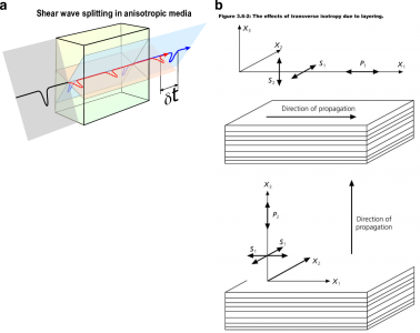
As well as showing lateral and vertical heterogeneities, the Earth is anelastic and anisotropic. Seismic waves are attenuated as they travel through the Earth, which affects observed amplitudes, and also makes wave velocity frequency dependent, which is known as dispersion (Fig. 4). Anisotropy causes waves to travel at different speeds dependent on their direction of travel or their polarization (Fig. 5). These properties are necessary features of reference models to properly represent seismic data. The first 1D reference model to include a realistic representation of attenuation, as well as radial anisotropy down to 200 km depth was PREM (Dziewonski and Anderson, 1981).

Figure 4 – The effect of anelasticity (attenuation) on wavespeed for a ‘standard linear solid’. This anelastic dispersion calculation demonstrates the need to account for anelasticity when comparing velocities across frequencies. a. Internal friction (attenuation) as a function of frequency for a band-limited "constant Q" model. b. Group and Phase velocities vary as a function of frequency due to attenuation c. Corresponding surface wave attenuation factor (energy lost per cycle) as a function of frequency demonstrating that the highest frequencies are the most strongly attenuated. From Liu et al., (1976).

Figure 5 - The effects of anisotropy on seismic waves. a. In anisotropic media, seismic wavespeeds depend on wave propagation direction and/or polarization. Travel through an anisotropic medium causes splitting of shear waves into a slow (red) and fast (blue) component. From garnero.asu.edu. b. In transversely anisotropic media, seismic waves travel at different velocities depending on their polarization and their propagation direction. Such a medium can be represented by 5 independent elastic parameters. PREM has transverse anisotropy in the upper mantle from the Moho (24.4 km) to 220 km depth. Figure 3.6.2 from Stein and Wysession (2009).

Limitations

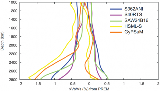
It should be stressed that 1D reference models are zeroth order approximations of the Earth structure (Fig. 1). In order to compute the travel times of seismic waves and compare them to real data, corrections due to earth's ellipticity that depend on the phase used need to be applied. The models often most poorly represent the uppermost and lowermost mantle where lateral velocity variations are strongest (Fig. 6). However, in the construction of these various models, authors are often explicit in stating the limitations of their products:

“An average Earth model, the subject of this work, is a mathematical abstraction. The lateral heterogeneity in the first few tens of kilometres is so large than an average model does not reflect the actual structure at any point.” - PREM (Dziewonski and Anderson, 1981, PEPI)

“It should be stressed that such a velocity model is intended as a summary of seismic travel-times and, because of the uneven geographic distribution of the ray paths sampled by the events in the ISC catalogue, will represent no simple average of the Earth.” – IASP91 (Kennett and Engdahl, 1991)

“We stress that model ak135 is designed to represent the smoother empirical travel-times, and so should be very suitable for predicting the arrival times of a wide variety of seismic phases for use in event location or phase association procedures. We have to be cautious about direct interpretation of ak135 as a full representation of seismic velocities in the Earth” AK135 - (Kennett et al., 1995)

Figure 6 – Velocity deviation of 3-D tomography models relative to PREM (1-D) averaged over the seismically slow (left lines) and fast (right lines) regions in the lower mantle for 5 different mantle tomographic models. PREM does not match the velocity structure of the 3-D models as it averages all lateral variations, thus it does not represent the velocity structure of any specific location and may not represent the properties of any real earth material. From Lekic et al., 2012.

Using models outside of seismology While it is useful to interpret the profiles with depth of elastic parameters in terms of composition and temperature, it is important to appreciate that they actually represent averages over heterogeneous structure. Therefore, care must be taken to not over interpret the model (Fig 7). Meanwhile, models differ hence selection of an appropriate model is important. For example, PREM was designed to dominantly fit whole Earth long period data (surface waves and normal modes) while also including body wave data, hence is best suited for comparison with other disciplines (Table 3).

Models are not equally well defined with depth for P- and S-waves as the regions that can be sampled depend on the phase (Kennett, 2006). Also, the accuracy of the travel-time measurements differs between P- and S-waves owing to the differences in dominant frequencies and contamination within the wavefield. Some chosen features of models make them incompatible with other data e.g. the choice of using linear gradients in AK135 mean that the model is unable to fit adiabat models (Kennett, 2006).

Reference models are usually defined in terms of P and S seismic velocities and density, from which elastic parameters can be inferred. Kennett (2006) argues that models should be defined as bulk and shear moduli and density for ease of comparison with mineral physics experiments. Similarly, tomography models are often described as the deviation from some 1D reference structure. While this makes displaying the structures simpler, any subsequent analysis of those structures will include the limitations inherent in the 1D model. Instead, using absolute velocities would prevent adding additional uncertainty to the data and thus not propagate into further analysis.

Figure 7. Mineral-physics predictions of seismic wave velocity for an Earth with a uniform bulk mantle composition, plotted relative to AK135. Uncertainties on the velocity model are shown as the grey shaded region. AK135 does not fit the calculated velocity structure of any material, most likely as it is a global average. Figure 1 from Matas et al (2007, GJI).

Summary of commonly used models While multiple reference models have been produced, there are three that have been most commonly used up to present: PREM (Dziewonski and Anderson, 1981), IASP91 (Kennett and Engdahl, 1991), and AK135 (Kennett et al., 1995). These models are summarised in Table 3 and their velocity structures are compared in Fig. 7. For more detail on these models, see section Common Models in Detail.

TABLE3 Table 3 – Summary of common reference models.

Whole mantle