
Model Overview (above)
There are three basic steps to our model:
- Model rupture to calculate the amount of heat generated
- One the heat is generated, allow it to conduct away from the fault
- Use time-temperature histories to calculate the effect of the heating event on fission track ages and track lengths.
1. Earthquake Energy Balance (below)
For our model of heat generation, we essentially follow the method outlined by Lachenbruch (1986). We start by computing the amount of heat generated by the earthquake, essentially invoking the formula for work from freshman physics (Work = Force * Distance).
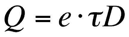
, where Q is the amount of heat generated per unit area of the fault, tau is the average shear stress, D is the total displacement during the earthquake, and e is an efficiency term. Tau is a force per unit area and D is a distance, so we get a work per unit area. However, not all of the work done during the earthquake is converted into heat. The illustration below shows the distribution of work into frictional heat generation, seismic wave radiation, and grain size reduction. While there is some debate over the magnitude of e, laboratory experiments (Lockner & Okubo, 1983) and calculations from seismic waveform spectra of real earthquakes (McGarr, 1999) both indicate that greater than 90% of earthquake work is converted into heat. We use 0.9 for e in our calculations. Also, Q, as expressed above, is the total heat. We assume that heat is distributed equally between the two sides of the fault, so Q for a one-dimensional heat conduction equation like we use below is one half the total heat.

Computing Shear Stress
We assume that shear stress is equal to an apparent coefficient of friction multiplied by the normal stress. In our forward model, we assumed values for the apparent coefficient of friction and determined the normal stress from the weight of the overburden. The apparent coefficient of friction includes the effects of pore pressure and the relative compressibility of the fault zone materials (Harris, 1998). Higher pore pressures will result in lower values of the apparent coefficient of friction, thus making the fault appear weaker.
2. Heat Transport
Because there are a number of unknowns about the rupture process, we make several simplifying assumptions. First, because the duration of slip is very short compared to the time of conduction we assume that all heat is generated instantaneously. Second, because the ultracataclasite layer at our sample locality is so narrow, we assume that heat is generated on an infinitely thin planar surface. This assumption is further supported by observations elsewhere on the San Gabriel fault and other exhumed faults by Chester that there is strong evidence for slip localizing along principal slip surfaces that are as thin as millimeters, even when the ultracataclasite/gouge layer is much wider.
The next assumption we make is that all heat transport is by conduction on the time scales of interest. While pore pressure gradients may be very high and permeability may increase during rupture (making fluid flow fairly rapid), there simply is not enough water present to carry away an appreciable amount of the heat. Even if fluids are moving around, during faulting, one likely scenario is that flow will be along the fault towards the surface. In that case, hot fluids from below will replace the heat transported away by pore fluids that are expelled during rupture. Both Lachenbruch (1980) and Mase and Smith (1986) who address the role of pore fluids in dynamically weakening faults ignore advective heat transport in their calculations. Further, Evans and Chester (1995) show that our specific sample locality has relatively little evidence for fluids or high fluid pressure. In other words, because of the short duration of high temperature pulses from individual earthquakes (minutes to hours), we feel that our estimates are insensitive to the heat transport by fluids. This stands in stark contrast to surface heat flow.
Solutions to the one-dimensional conduction equation for an instantaneous plane source of heat are common in some of the famous references such as Carslaw and Jaeger (1959) and Ingersoll et al. (1954):

When this equation is plotted for typical conditions for an earthquake at the depth of interest for this study, the time-temperature history produces an extremely localized temperature pulse. Note that only areas within about 10 cm of the fault surface are ever exposed to temperature increases greater than 100 degrees C, and that these temperatures only persist for less than an hour.
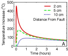
Parameters: Depth, 2.3 km; Slip, 4m; Apparent coefficient of friction, 0.35